3 Excel Formulas for Google’s Keyword Planner Search Volume Numbers
3 Excel Formulas for Google’s Keyword Planner Search Volume Numbers
Our main sources of keyword data, no matter what keyword research tools we use, is oftentimes Google’s Keyword Planner, which is a part of Google AdWords. Data from Keyword Planner is exported into CSV files or extracted using their API to feed other tools.
Google has a history of being less transparent, no matter what kind of data or tool. See 100% not provided in Google Analytics incoming keyword traffic; removing archived data in Google Search Console aka Webmaster Tools and just keeping the last 90 days; and using large ranges of search volume numbers in Google Adwords Keyword Planner.
Aside from using large rounded-off search volume numbers, the ranges are saved in the same column separated by a dash, and using K and M instead of adding actual digits for the thousand and million factors. So once exported and opened in your online spreadsheet, you will get values like this:
- 0 – 10
- 10 – 100
- 100 – 1K
- 1K – 10K
- 10K – 100K
- 100K – 1M
- 1M – 20M
Having values like that in a single spreadsheet column are not that usable if you ever use the numbers for some additional calculations. Even sorting them largest to smallest is not possible.
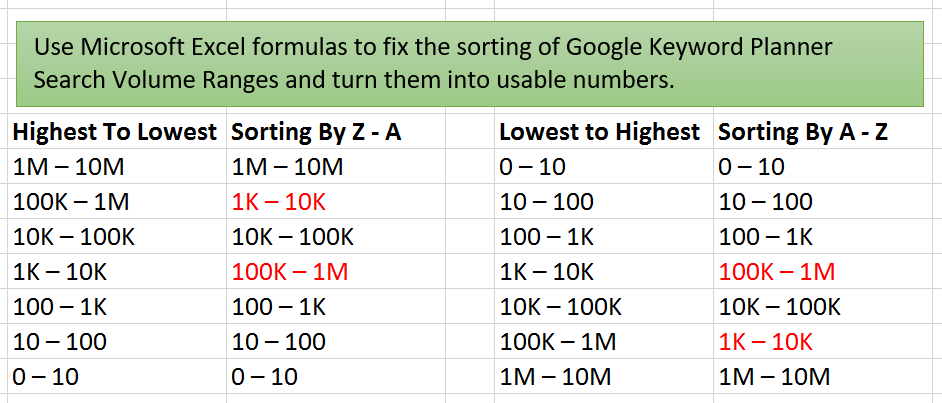
There are some people that use search volume to compute for the keyword effectiveness index or KEI. Different people change these range of values from text strings to actual numbers by doing some find and replace methods, using regex, some within Excel, some using HTML editors, some using scripting languages like Python or R. Here I present you with a formula to pull out the numbers using Excel that is easy to copy and paste.
Excel Formula for Displaying Google’s Keyword Planner Search Volume Ranges as Normal Numbers
Some of us want to understand the how and why of these formulas. If you are not interested in that and just need the formulas, then scroll down to the end of this blog post.
Since this is a range of numbers, you are turning one column into two columns — the start of the range and the end of the range — and in some cases, you may want to just get the average. I will present three formulas for minimum, maximum, and average search volume.
Extracting the Minimum Search Volume Number
Before extracting the minimum and maximum, let’s take care of the “K” and “M” first and convert them to “000” and “000000” respectively. We can do a text string replacement with the SUBSTITUTE formula. Assuming the search volume range is in cell B2, use the formula below:
=SUBSTITUTE(B2,"K","000")
What should appear by now on your spreadsheet would be something like this:
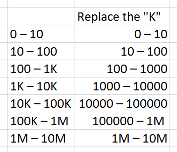
Using the same formula, you can nest in the replacement of “M”. To easily see what was added in the formula, I used a different color.
=SUBSTITUTE(SUBSTITUTE(B2,"K","000"),"M","000000")
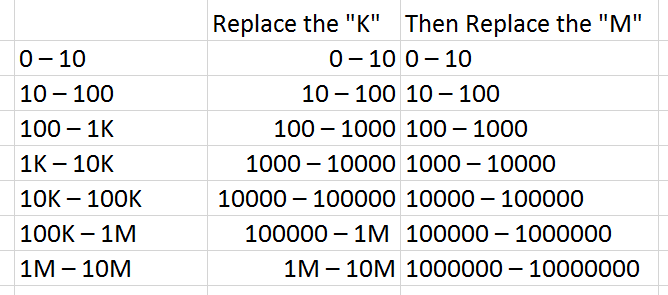
This takes care of all the Ks and Ms. The next formula is just about getting the first number and the last number. The minimum number is the number of left, and this can be done with the formula LEFT, but you need to specify how long the string is.
=LEFT(SUBSTITUTE(SUBSTITUTE(B2,"K","000"),"M","000000"),3)
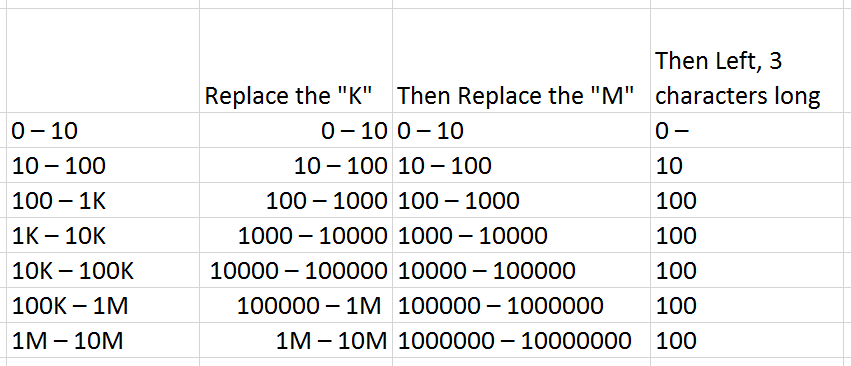
With the number 3, it will only get the first 3 characters. So, this will only work for 100, and for nothing else.
We can find the required length of the string by looking at the position of the “–“, and to find this position, you can use the Excel formula FIND and subtract the spaces.
=LEFT(SUBSTITUTE(SUBSTITUTE(B2,"K","000"),"M","000000"),
 FIND("–",SUBSTITUTE(SUBSTITUTE(B2,"K","000"),"M","000000"))-2)
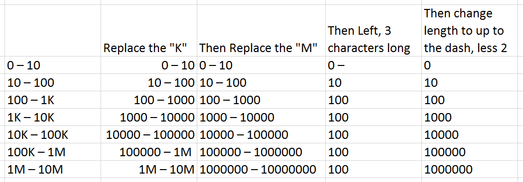
Important Note: Be careful in finding the “–“ in the formula. If it is not working, you might be using the en-dash and not the em-dash. They both look the same, but the em-dash is longer. (For me to easily remember, the en-dash has the width of an “n” and an em-dash has the width of an “m.” If you don’t know how to make the em-dash come out, then just try copy and pasting from the exported file from Google Keyword Planner.
This formula already works and you can use its value in other computations, but sometimes it can still cause errors in sorting if spaces are appended to the numbers. To convert the text string to numbers, just use NUMBERVALUE.
=NUMBERVALUE(
 LEFT(SUBSTITUTE(SUBSTITUTE(B2,"K","000"),"M","000000"),
 FIND("–",SUBSTITUTE(SUBSTITUTE(B2,"K","000"),"M","000000"))-2))

Extracting the Maximum Search Volume Number
Since we already changed the “K” and “M” in the previous exercise, we will start from there. Assuming again that the search volume range is in cell B2, use the formula below:
=SUBSTITUTE(SUBSTITUTE(B2,"K","000"),"M","000000")
This time we do not need the number on the left of the “-“, it should be on the right. So we use right instead. And temporarily, I made the text string a length of 3 again to learn this step-by-step.
=RIGHT(SUBSTITUTE(SUBSTITUTE(B2,"K","000"),"M","000000"),3)
Like the formula for getting the minimum value, we look for the hyphen using FIND, but remember, the number it returns is the position of the dash from the left. But at the dash position, the number of characters on the left is just 1 character less (less zeroes) and one character more (for the dash itself) and should be equal to the number of characters on the right. Thus, unlike the formula for the minimum, you see no “-2” after the find.
=RIGHT(SUBSTITUTE(SUBSTITUTE(B2,"K","000"),"M","000000"),
 FIND("–",SUBSTITUTE(SUBSTITUTE(B2,"K","000"),"M","000000")))
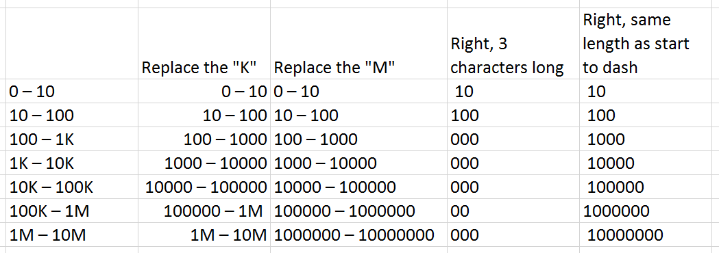
Since the right of the dash has a space, you will see a space before each number except for one of them. This is still in text form, and once you change them to numbers with NUMBERVALUE, the spaces do not matter.
=NUMBERVALUE(
 RIGHT(SUBSTITUTE(SUBSTITUTE(B2,"K","000"),"M","000000"),
 FIND("–",SUBSTITUTE(SUBSTITUTE(B2,"K","000"),"M","000000"))))

Extracting the Average Search Volume Number
If you prefer to use the average of the range, we simply need to add these and divide it by two. This now sums up all 3 formulas you will need to convert the search volume text string ranges.
Excel Formula #1: Google Keyword Planner Minimum Search Volume
=NUMBERVALUE(
 LEFT(SUBSTITUTE(SUBSTITUTE(B2,"K","000"),"M","000000"),
 FIND("–",SUBSTITUTE(SUBSTITUTE(B2,"K","000"),"M","000000"))-2))
Excel Formula #2: Google Keyword Planner Maximum Search Volume
=NUMBERVALUE(
 RIGHT(SUBSTITUTE(SUBSTITUTE(B2,"K","000"),"M","000000"),
 FIND("–",SUBSTITUTE(SUBSTITUTE(B2,"K","000"),"M","000000"))))
Excel Formula #3: Google Keyword Planner Average Search Volume
The average should be self-explanatory from there. But be sure to use some extra parenthesis in there to make sure the operation happens in the right order.
The average number is:
=(NUMBERVALUE(
 LEFT(SUBSTITUTE(SUBSTITUTE(B2,"K","000"),"M","000000"),
 FIND("–",SUBSTITUTE(SUBSTITUTE(B2,"K","000"),"M","000000"))-2)) +
 NUMBERVALUE(
 RIGHT(SUBSTITUTE(SUBSTITUTE(B2,"K","000"),"M","000000"),
 FIND("–",SUBSTITUTE(SUBSTITUTE(B2,"K","000"),"M","000000")))))/2
Now that you have all values as numbers you can use them for any calculations, computing it with KEI, or with other numbers that makes the most sense to you.


Nessun commento: